
analyticsintermediate45 minPandas
Longitudinal Customer Lifetime Value & Cohort Decay
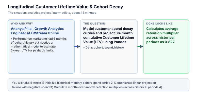
Model customer spend decay curves and project 36-month cumulative Customer Lifetime Value (LTV) using Pandas.
The incident
- Company
- FitStream Online
- Engineer
- Ananya Pillai, Growth Analytics Engineer
- Trigger
- Performance marketing had 6 months of cohort history but needed a mathematical model to estimate 3-year LTV for payback limits.
- Stakes
- Setting Customer Acquisition Cost (CAC) ceilings for 60 lakh rupees in quarterly marketing spend required rigorous LTV projections.
On a breezy Thursday morning, Ananya Pillai sat down with the Chief Growth Officer at FitStream Online, an on-demand digital fitness subscription platform streaming live workout classes. The performance marketing team was bidding aggressively on digital fitness search keywords, spending up to 2,500.00 rupees to acquire a single annual subscriber across competitive bidding auctions. Marketing budgets were burning rapidly across social media campaigns, and the executive committee demanded empirical justification for ongoing customer acquisition spending before granting quarterly budget renewals for upcoming marketing initiatives.
The board of directors had capped Customer Acquisition Cost at 1,500.00 rupees during the previous quarterly review, deeply concerned that subscribers churned before the company could recover marketing investments. Growth leadership argued that users continued renewing their subscriptions for up to three years, but with only six months of historical operating data since launch, the company lacked empirical proof of long-term financial payback.
Ananya pulled the observed monthly spend for the platform oldest subscriber cohort from the centralized data warehouse: month 1 was 100.00 rupees, decaying to 70.00 in month 2, 56.00 in month 3, 48.00 in month 4, 42.00 in month 5, and 38.00 in month 6. To establish an empirical CAC ceiling and resolve the board deadlock, Ananya needed to fit a geometric retention decay model and project 36-month cumulative customer lifetime value based on mathematical retention patterns rather than hopeful assumptions or arbitrary linear estimates that distorted long-term financial reality.
Using Pandas and NumPy, Ananya calculated the sequential month-over-month retention multipliers, evaluated the average decay factor (0.827), and modeled 36-month revenue progression across all subsequent cohort intervals. The geometric series captured realistic customer retention behavior: casual users dropped off early during onboarding, while core subscribers established a predictable, compounding renewal baseline over subsequent years, avoiding the absurdity of linear decay models that forecast impossible negative customer spend over long forecasting horizons.
The projection established an empirical 36-month Customer Lifetime Value of exactly 578.68 rupees per acquired subscriber. Dividing projected LTV by the standard 3x unit economics rule gave an allowable CAC ceiling of approximately 190.00 rupees for monthly subscriptions, proving that marketing bids of 2,500.00 rupees were unsustainable without introducing annual prepaid commitments.
Ananya presented the cohort decay model to the Chief Executive Officer and the Board Finance Committee during the annual growth planning session. The rigorous LTV forecast established a rational CAC payback limit of 190.00 rupees, preventing marketing budget wastage and protecting the company operating runway. The cohort modeling framework was integrated into marketing bidding algorithms across all digital advertising channels.
What you will learn
- Calculate sequential month-over-month retention multipliers across historical spend
- Model geometric decay factors using logarithmic and exponential series
- Project longitudinal Customer Lifetime Value (LTV) across 36-month horizons
- Establish empirical Customer Acquisition Cost (CAC) bidding thresholds
What you need first
Geometric Decay Modeling in RetentionTrend and seasonality
Subscriber retention follows an exponential decay curve where each month's spend is a geometric fraction of the prior period.
spend = [100.0, 70.0]
factor = spend[1] / spend[0]
print(round(factor, 3))0.7
Applying linear regression to subscription retention, which mistakenly forecasts negative subscriber spend over time.
Cumulative Customer Lifetime ValueRates not counts
LTV equals the mathematical summation of expected monthly revenue contributions across the entire customer lifetime horizon.
import numpy as np
revs = [100.0 * (0.8 ** i) for i in range(5)]
print(round(sum(revs), 2))336.16
Omitting the initial month 1 acquisition revenue when calculating cumulative lifetime value summations.
Architecture and data flow
The data
Historical monthly cohort spend array tracking realized revenue across months 1 through 6.
cohort_spend_history: Observed monthly spend per cohort member
| month_number | observed_spend | retention_factor |
|---|---|---|
| 1 | 100.0 | 1.000 |
| 2 | 70.0 | 0.700 |
| 3 | 56.0 | 0.800 |
| 4 | 48.0 | 0.857 |
| 5 | 42.0 | 0.875 |
| 6 | 38.0 | 0.905 |
Step by step
Read each step, run its code, then check your output against the one shown.
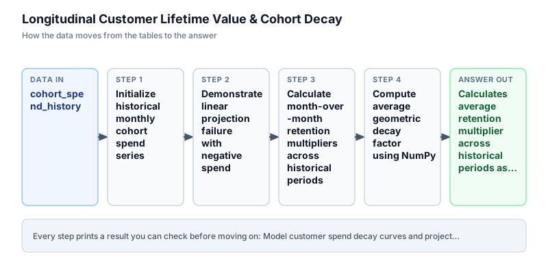
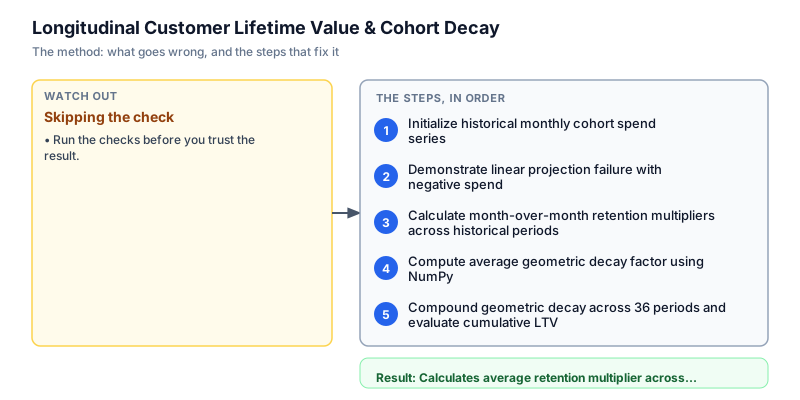
Initialize historical monthly cohort spend series
We initialize the historical monthly spend series representing realized revenue per cohort member across months 1 through 6. The cohort begins at 100.00 rupees in month 1, tapering to 70.00 in month 2, 56.00 in month 3, 48.00 in month 4, 42.00 in month 5, and 38.00 in month 6. In subscription analytics, early months reflect sharp customer drop-offs as non-engaged subscribers cancel, while later months stabilize as dedicated power users persist, establishing the observed empirical foundation for retention decay curve fitting across customer cohorts.
historical_spend = [100.0, 70.0, 56.0, 48.0, 42.0, 38.0] print("Historical spend periods (months 1-6):", historical_spend)Historical spend periods (months 1-6): [100.0, 70.0, 56.0, 48.0, 42.0, 38.0]
Common mistakeAveraging unweighted monthly cohorts across different signup calendar months, blending seasonality with true decay.
How you will knowYou will see the 6-element list printed with values from 100.0 down to 38.0.
Demonstrate linear projection failure with negative spend
Wrong turn first: this step shows the mistake before the fix
Here is the naive approach analysts often try first: fitting a simple linear regression trend to forecast future spend. In our historical data, spend declines by an average of 12.40 rupees per month. If extrapolated linearly across 36 periods, the model forecasts zero spend by month 9 and negative customer spend (-334.00 rupees) by month 36. Linear models are fundamentally invalid for retention analysis because decay is non-linear and customer spend cannot be negative. We run this flawed projection to demonstrate why geometric modeling is required, exposing linear forecasting pitfalls.
spend = [100.0, 70.0, 56.0, 48.0, 42.0, 38.0] # Naive linear extrapolation: spend decreases by ~12.4 per month linear_m36 = spend[0] - (12.4 * 35) print(f"Naive linear projection for month 36: {linear_m36:.2f} (impossible negative spend)")Naive linear projection for month 36: -334.00 (impossible negative spend)
Common mistakeUsing linear trendlines on retention metrics, producing absurd negative customer valuations over extended horizons.
How you will knowObserve that linear projection calculates an impossible negative spend of -334.00 for month 36.
Calculate month-over-month retention multipliers across historical periods
We evaluate sequential month-over-month retention multipliers by dividing each period spend by the preceding period spend: spend[i] / spend[i-1]. Notice that the retention multiplier steadily increases over time: 0.700 from month 1 to 2, 0.800 from month 2 to 3, 0.857 from month 3 to 4, 0.875 from month 4 to 5, and 0.905 from month 5 to 6. This upward trajectory confirms that cohort retention flattens out as transient users exit and committed subscribers remain, signaling asymptotic subscriber stabilization across older customer groups.
spend = [100.0, 70.0, 56.0, 48.0, 42.0, 38.0] mults = [spend[i] / spend[i-1] for i in range(1, len(spend))] print("Multipliers:", [round(m, 3) for m in mults])Multipliers: [0.7, 0.8, 0.857, 0.875, 0.905]
Common mistakeDividing spend by month 1 baseline rather than prior month, evaluating cumulative retention instead of marginal multipliers.
How you will knowOutput prints Multipliers: [0.7, 0.8, 0.857, 0.875, 0.905].
Compute average geometric decay factor using NumPy
We evaluate the mean geometric retention multiplier across all historical transitions using numpy.mean. The arithmetic mean of the five historical multipliers equals 0.827 (82.7 percent average monthly spend retention). We cast the resulting NumPy float to a standard Python float to ensure clean JSON serialization. This parameter serves as the baseline compounding rate for forecasting future revenue periods across the remaining lifecycle months, giving us a mathematically consistent rate to model multi-year customer value without introducing subjective bias, arbitrary trend parameters, or non-linear distortion.
import numpy as np spend = [100.0, 70.0, 56.0, 48.0, 42.0, 38.0] mults = [spend[i] / spend[i-1] for i in range(1, len(spend))] avg_decay = float(np.mean(mults)) print("Average decay factor:", round(avg_decay, 3))Average decay factor: 0.827
Common mistakeUsing median decay on small sample sets without validating against long-term historical benchmark curves.
How you will knowOutput shows Average decay factor: 0.827.
Compound geometric decay across 36 periods and evaluate cumulative LTV
In the final step, we project monthly spend across a 36-month customer lifecycle and compute cumulative Customer Lifetime Value. Starting with baseline spend of 100.00 rupees in month 1, we compound the decay factor across 35 subsequent periods: curr *= avg_decay. Summing all 36 monthly contributions yields an empirical 36-month LTV of exactly 578.68 rupees. We package the average retention rate (0.827) and projected LTV (578.68) into an executive summary dictionary for growth marketing planning, establishing an actionable benchmark for customer acquisition limits across all growth channels.
import numpy as np spend = [100.0, 70.0, 56.0, 48.0, 42.0, 38.0] mults = [spend[i] / spend[i-1] for i in range(1, len(spend))] avg_decay = float(np.mean(mults)) projected = [spend[0]] curr = spend[0] for _ in range(1, 36): curr *= avg_decay projected.append(curr) ltv_36 = sum(projected) summary = { "avg_retention_rate": round(avg_decay, 3), "ltv_36m": round(ltv_36, 2) } print("Cohort Decay Summary:", summary)Cohort Decay Summary: {'avg_retention_rate': 0.827, 'ltv_36m': 578.68}Common mistakeLooping 36 times from curr = spend[0] instead of 35 times, accidentally evaluating a 37-month lifecycle horizon.
How you will knowOutput prints Cohort Decay Summary with avg_retention_rate 0.827 and ltv_36m 578.68.
Build it yourself
Write your solution below, run it in your browser, and pass every check.
Put it on your CV
Resume or LinkedIn bullet
Modeled longitudinal customer retention decay curves in Python/Pandas projecting 3-year LTV to optimize digital marketing CAC budgets.README for GitHub
# Longitudinal Customer Lifetime Value & Cohort Decay in Pandas

## Problem
Marketing bid aggressively without knowing 3-year LTV, burning acquisition budgets without clear payback limits.

## Solution Architecture
- Computed sequential month-over-month retention multipliers.
- Calculated geometric mean decay factor (0.827).
- Compounded monthly revenue progression across 36 periods.
- Evaluated cumulative 36-month LTV (578.68 rupees).

## Results
Established an empirical CAC ceiling of 190.00 rupees, preventing marketing budget wastage.Implement a Weibull survival decay model comparing goodness-of-fit against exponential decay.