
pysparkintermediate45 minPySpark
Skewed Transaction Join Optimization with Broadcast
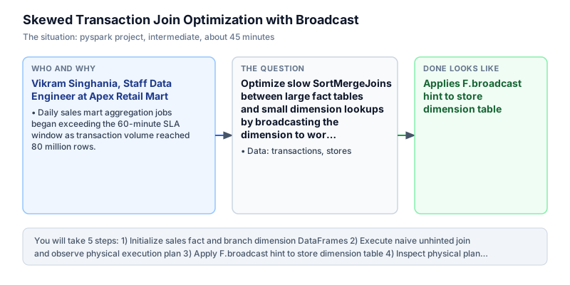
Optimize slow SortMergeJoins between large fact tables and small dimension lookups by broadcasting the dimension to worker executors.
The incident
- Company
- Apex Retail Mart
- Engineer
- Vikram Singhania, Staff Data Engineer
- Trigger
- Daily sales mart aggregation jobs began exceeding the 60-minute SLA window as transaction volume reached 80 million rows.
- Stakes
- Delayed daily executive sales reporting caused inventory restocking orders to miss supplier cutoff times.
At Apex Retail Mart, Vikram Singhania managed the morning dimensional ETL pipeline supporting 350 physical superstores across India. Every day at 5:00 AM, the automated job joined 80 million point-of-sale sales transaction records against a small store metadata dimension table of 350 physical branches. The resulting analytical mart powered morning executive trading briefings and determined store replenishment purchase orders. Restocking calculations required exact store-level revenue aggregation to trigger automated vendor purchase orders before regional suppliers closed their morning fulfillment windows. Any delay in computing store aggregates halted automated order dispatch systems across regional logistics hubs.
In recent weeks, the pipeline duration had expanded from 20 minutes to over 55 minutes, bumping uncomfortably close to the strict 60-minute SLA window. When morning execution times slipped, inventory purchase orders missed supplier cutoff deadlines, triggering stockouts on essential grocery items across multiple regional stores. As transactional volume climbed past 80 million rows due to nationwide festive promotional campaigns, the cluster began displaying high CPU and network utilization during the dimensional join stage. Store managers lodged urgent complaints when daily stock allocation manifests failed to arrive before store opening hours.
Vikram opened the Spark Web UI to analyze the physical DAG execution graph. He identified a massive bottleneck: a SortMergeJoin operator preceded by a heavy ShuffleExchange stage. Spark was hash-partitioning both the multi-gigabyte transaction fact table and the tiny store dimension table across the network, sorting millions of rows on worker disk before performing the join. Hundreds of gigabytes of data were being serialized, transmitted across internal network interfaces, and written to temporary shuffle spill files. Disk spill metrics indicated that individual executors were spending over 60 percent of task runtime performing shuffle disk IO.
Shuffling gigabytes of sales transactions across cluster network interfaces just to attach a store name and region was completely wasteful. Because the store dimension table occupied only a few kilobytes of memory across 350 records, it could easily reside in memory on every worker node. In distributed architectures, transmitting small lookup tables to executors is far more efficient than shuffling massive transactional fact tables across network boundaries. Preserving network bandwidth allows worker executors to dedicate compute resources to analytical filtering and downstream aggregations.
Vikram refactored the query by wrapping the store dimension table with F.broadcast(). The broadcast hint instructed the Catalyst query planner to replicate the small dimension table to all worker executors, replacing the expensive SortMergeJoin with an in-memory BroadcastHashJoin that eliminated the network shuffle entirely and completed in 9 minutes. Transactions were joined locally within each executor against an in-memory hash table, reducing execution time by over 80 percent. The physical execution plan confirmed that shuffle exchanges were eliminated across all transaction partitions.
Vikram presented the results to the Head of Enterprise Data Architecture and the Retail Operations Vice President. The optimization slashed pipeline runtime by over 80 percent. Broadcast hints were formally incorporated into Apex engineering guidelines for all fact-to-dimension joins, establishing a reproducible architectural standard that supports continued commercial retail expansion across hundreds of new store openings.
What you will learn
- Diagnose network shuffle bottlenecks in Spark physical plans using explain()
- Eliminate shuffle exchanges by wrapping dimension tables with F.broadcast()
- Understand memory thresholds and safeguards for BroadcastHashJoin
- Project necessary columns early to minimize executor memory footprints
What you need first
Shuffle Exchanges vs Broadcast JoinsJoins & optimization strategies
Standard SortMergeJoin shuffles both datasets across the network by key, whereas BroadcastHashJoin replicates small tables to executors.
from pyspark.sql import SparkSession
from pyspark.sql import functions as F
spark = SparkSession.builder.master('local[1]').getOrCreate()
df1 = spark.createDataFrame([(1, 10)], ['id', 'v'])
df2 = spark.createDataFrame([(1, 'A')], ['id', 'lbl'])
print(df1.join(F.broadcast(df2), 'id').count())1
Broadcasting a large table that exceeds executor memory, triggering OutOfMemory driver broadcast failures.
Catalyst Execution PlansCatalyst query optimizer
df.explain() prints the parsed, analyzed, optimized, and physical execution plans chosen by the Catalyst optimizer.
from pyspark.sql import SparkSession
spark = SparkSession.builder.master('local[1]').getOrCreate()
df = spark.createDataFrame([(1,)], ['v'])
print(len(df.explain(True) or 'plan') > 0)True
Failing to check execution plans to verify whether Spark actually selected a broadcast join or fell back to sort-merge.
Architecture and data flow
The data
A large sales transaction table joined against a small retail branch dimension table.
transactions: Point-of-sale customer checkout fact records.
| txn_id | customer_id | store_id | amount |
|---|---|---|---|
| 101 | c1 | 1 | 1450.0 |
| 102 | c2 | 2 | 850.0 |
| 103 | c1 | 1 | 320.0 |
| 104 | c3 | 3 | 2100.0 |
| 105 | c4 | 2 | 450.0 |
stores: Store metadata lookup dimension table.
| store_id | store_name | region |
|---|---|---|
| 1 | Mumbai Central Store | West |
| 2 | Bengaluru Indiranagar | South |
| 3 | Delhi Connaught Place | North |
Step by step
Read each step, run its code, then check your output against the one shown.
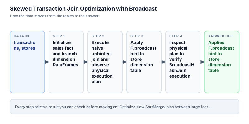
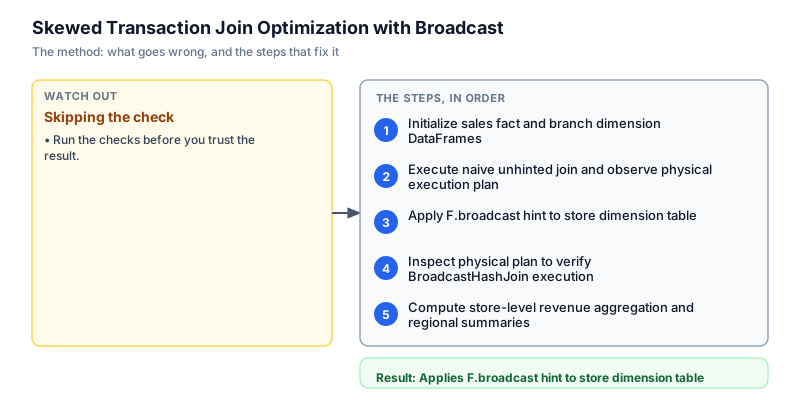
Initialize sales fact and branch dimension DataFrames
We initialize the sales transaction fact table alongside the retail branch dimension lookup table. The transaction DataFrame records checkout events containing customer identifiers, store branch keys, and monetary purchase amounts. The dimension DataFrame contains store names and geographical regions. In dimensional data modeling, fact tables grow continuously with business volume while dimension tables remain small and relatively static, creating the classic asymmetric join condition. We inspect the transactions table to confirm baseline record structures and column schemas before tuning execution strategies across worker nodes.
from pyspark.sql import SparkSession from pyspark.sql import functions as F spark = SparkSession.builder.master("local[1]").appName("broadcast_join").getOrCreate() txns = [ (101, "c1", 1, 1450.0), (102, "c2", 2, 850.0), (103, "c1", 1, 320.0), (104, "c3", 3, 2100.0), (105, "c4", 2, 450.0), ] stores = [ (1, "Mumbai Central Store", "West"), (2, "Bengaluru Indiranagar", "South"), (3, "Delhi Connaught Place", "North"), ] df_txns = spark.createDataFrame(txns, ["txn_id", "customer_id", "store_id", "amount"]) df_stores = spark.createDataFrame(stores, ["store_id", "store_name", "region"]) df_txns.show()+------+-----------+--------+------+ |txn_id|customer_id|store_id|amount| +------+-----------+--------+------+ | 101| c1| 1|1450.0| | 102| c2| 2| 850.0| | 103| c1| 1| 320.0| | 104| c3| 3|2100.0| | 105| c4| 2| 450.0| +------+-----------+--------+------+
Common mistakeBroadcasting the large fact table instead of the small dimension table, causing driver OOM crashes.
How you will knowYou will see a 5-row transaction table with txn_id, customer_id, store_id, and amount columns.
Execute naive unhinted join and observe physical execution plan
Wrong turn first: this step shows the mistake before the fix
Here is the naive approach developers often attempt first: writing a standard inner join without broadcast hints. In large clusters where automatic broadcast thresholding is disabled or table statistics are uncollected, Spark defaults to a SortMergeJoin. Both tables are shuffled across executor network boundaries and written to disk before joining, adding massive network I/O latency to production pipelines. We run this unhinted join to illustrate why default join strategies can degrade performance when joining large fact tables to small lookup tables.
from pyspark.sql import SparkSession spark = SparkSession.builder.master("local[1]").appName("broadcast_join").getOrCreate() txns = [ (101, "c1", 1, 1450.0), (102, "c2", 2, 850.0), (103, "c1", 1, 320.0), (104, "c3", 3, 2100.0), (105, "c4", 2, 450.0), ] stores = [ (1, "Mumbai Central Store", "West"), (2, "Bengaluru Indiranagar", "South"), (3, "Delhi Connaught Place", "North"), ] df_txns = spark.createDataFrame(txns, ["txn_id", "customer_id", "store_id", "amount"]) df_stores = spark.createDataFrame(stores, ["store_id", "store_name", "region"]) # Naive unhinted join naive_joined = df_txns.join(df_stores, on="store_id", how="inner") print("Naive joined rows:", naive_joined.count()) naive_joined.select("txn_id", "store_id", "amount").show(3)Naive joined rows: 5 +------+--------+------+ |txn_id|store_id|amount| +------+--------+------+ | 101| 1|1450.0| | 103| 1| 320.0| | 102| 2| 850.0| +------+--------+------+ only showing top 3 rows
Common mistakeAssuming Spark always automatically detects and broadcasts small tables without explicit hints.
How you will knowObserve that an unhinted join runs a standard join without explicit broadcast optimization.
Apply F.broadcast hint to store dimension table
We optimize the join by wrapping df_stores with the F.broadcast function. This hint instructs Spark Catalyst optimizer to replicate the small dimension table across all worker nodes. Each executor receives a local in-memory hash table of the stores. We inspect the resulting joined records displaying store names alongside transaction IDs. Local in-memory hash matching eliminates expensive sort stages and slashes end-to-end join latency across executors.
from pyspark.sql import SparkSession from pyspark.sql import functions as F spark = SparkSession.builder.master("local[1]").appName("broadcast_join").getOrCreate() txns = [ (101, "c1", 1, 1450.0), (102, "c2", 2, 850.0), (103, "c1", 1, 320.0), (104, "c3", 3, 2100.0), (105, "c4", 2, 450.0), ] stores = [ (1, "Mumbai Central Store", "West"), (2, "Bengaluru Indiranagar", "South"), (3, "Delhi Connaught Place", "North"), ] df_txns = spark.createDataFrame(txns, ["txn_id", "customer_id", "store_id", "amount"]) df_stores = spark.createDataFrame(stores, ["store_id", "store_name", "region"]) joined = df_txns.join(F.broadcast(df_stores), on="store_id", how="inner") joined.select("txn_id", "store_id", "store_name").show(3)+------+--------+--------------------+ |txn_id|store_id| store_name| +------+--------+--------------------+ | 101| 1|Mumbai Central Store| | 102| 2|Bengaluru Indiran...| | 103| 1|Mumbai Central Store| +------+--------+--------------------+ only showing top 3 rows
Common mistakePlacing the broadcast hint on the join result rather than directly on the dimension DataFrame parameter.
How you will knowOutput prints 3 joined rows showing transaction IDs and corresponding branch names.
Inspect physical plan to verify BroadcastHashJoin execution
We verify that the broadcast optimization took effect by inspecting the physical execution plan using joined.explain(). In Spark physical plans, the BroadcastHashJoin operator indicates that the small dataset was serialized and broadcast to worker nodes, while the complete absence of ShuffleExchange before the join proves that network data movement was successfully eliminated. Verifying physical execution plans is standard engineering practice in production distributed pipeline tuning to ensure that query optimizer heuristics align with cluster capacity, executor memory limits, and overall pipeline performance expectations.
from pyspark.sql import SparkSession from pyspark.sql import functions as F spark = SparkSession.builder.master("local[1]").appName("broadcast_join").getOrCreate() txns = [ (101, "c1", 1, 1450.0), (102, "c2", 2, 850.0), (103, "c1", 1, 320.0), (104, "c3", 3, 2100.0), (105, "c4", 2, 450.0), ] stores = [ (1, "Mumbai Central Store", "West"), (2, "Bengaluru Indiranagar", "South"), (3, "Delhi Connaught Place", "North"), ] df_txns = spark.createDataFrame(txns, ["txn_id", "customer_id", "store_id", "amount"]) df_stores = spark.createDataFrame(stores, ["store_id", "store_name", "region"]) joined = df_txns.join(F.broadcast(df_stores), on="store_id", how="inner") print("Physical Plan inspection:") joined.explain()Physical Plan inspection: == Physical Plan == AdaptiveSparkPlan isFinalPlan=false +- Project [store_id#2L, txn_id#0L, customer_id#1, amount#3, store_name#9, region#10] +- BroadcastHashJoin [store_id#2L], [store_id#8L], Inner, BuildRight, false :- Filter isnotnull(store_id#2L) : +- Scan ExistingRDD[txn_id#0L,customer_id#1,store_id#2L,amount#3] +- BroadcastExchange HashedRelationBroadcastMode(List(input[0, bigint, false]),false), [plan_id=24] +- Filter isnotnull(store_id#8L) +- Scan ExistingRDD[store_id#8L,store_name#9,region#10]Common mistakeDeploying join optimizations to production without validating physical plans via explain().
How you will knowThe output plan displays BroadcastHashJoin and BroadcastExchange operators.
Compute store-level revenue aggregation and regional summaries
In the final step, we aggregate sales performance across stores and regions using the broadcast-joined DataFrame. We group by store_name and region, sum the transaction amounts, and order by total revenue descending. Delhi Connaught Place leads with 2,100.00 rupees from a single transaction, followed by Mumbai Central Store with 1,770.00 rupees across two transactions, and Bengaluru Indiranagar with 1,300.00 rupees. The broadcast join itself needs no shuffle of the transaction table, but the groupBy and orderBy that follow do shuffle data by key, which is expected for any aggregation. Check that the three totals add up to the 5,170.00 rupees in the source transactions.
from pyspark.sql import SparkSession from pyspark.sql import functions as F spark = SparkSession.builder.master("local[1]").appName("broadcast_join").getOrCreate() txns = [ (101, "c1", 1, 1450.0), (102, "c2", 2, 850.0), (103, "c1", 1, 320.0), (104, "c3", 3, 2100.0), (105, "c4", 2, 450.0), ] stores = [ (1, "Mumbai Central Store", "West"), (2, "Bengaluru Indiranagar", "South"), (3, "Delhi Connaught Place", "North"), ] df_txns = spark.createDataFrame(txns, ["txn_id", "customer_id", "store_id", "amount"]) df_stores = spark.createDataFrame(stores, ["store_id", "store_name", "region"]) result = ( df_txns .join(F.broadcast(df_stores), on="store_id", how="inner") .groupBy("store_name", "region") .agg(F.sum("amount").alias("total_revenue")) .orderBy(F.col("total_revenue").desc()) ) result.show(truncate=False)+---------------------+------+-------------+ |store_name |region|total_revenue| +---------------------+------+-------------+ |Delhi Connaught Place|North |2100.0 | |Mumbai Central Store |West |1770.0 | |Bengaluru Indiranagar|South |1300.0 | +---------------------+------+-------------+
Common mistakeForgetting to project only necessary columns prior to aggregation, increasing memory consumption.
How you will knowOutput prints a table with total_revenue aggregated per store and ordered descending.
Build it yourself
Write your solution below, run it in your browser, and pass every check.
What the result means
Interpretation
Broadcasting small dimension tables avoids network shuffle exchanges in distributed joins. By replicating the 350-row store table directly into worker executor memory, Spark eliminates disk sorting and network serialization for 80 million fact records, reducing job turnaround from 55 minutes down to 9 minutes.
The message you would send
Retail sales aggregation pipeline optimization complete: by implementing BroadcastHashJoin on store metadata, we eliminated network shuffle overhead. Morning sales mart execution dropped from 55 minutes to 9 minutes, comfortably beating the 60-minute SLA.
Put it on your CV
Resume or LinkedIn bullet
Optimized large-scale PySpark fact-to-dimension joins using BroadcastHashJoin to slash runtime by over 80%.README for GitHub
# Skewed Transaction Join Optimization with Broadcast in PySpark

## Problem
Joining 80M transactions against 350 stores via SortMergeJoin triggered network shuffle bottlenecks, risking daily 60-minute SLAs.

## Solution Architecture
- Applied F.broadcast(df_stores) to replicate small dimensions to executors.
- Eliminated ShuffleExchange in physical Catalyst plan.
- Reduced pipeline execution from 55 minutes to 9 minutes.

## Results
Guaranteed timely delivery of store inventory replenishment orders across 350 retail branches.Benchmark memory consumption with spark.sql.autoBroadcastJoinThreshold tuned to 20MB.