
Overview
One country owning most rows is a straggler. Salt the hot key so the crew can share the pallet.
On this page8 sections
The broken result
Say a Spark job that used to take minutes now takes an hour. The stage sits at 99% while one task keeps running.
What does the stall look like?
Take a made-up table of 1,000 shop events. Most come from one country.
A straggler is the one slow task. The whale is the key far bigger than the rest.
If IN appears in most rows, a groupBy country will not be even work.
A groupBy on country sends every IN row to the same task. The other tasks finish and wait.
Skew means one key holds far more rows than its siblings.
Why does the whole job wait for one task?
A stage ends when its slowest task, the straggler, ends. The job time is that task, not the average.
Predict before you step: do you add executors, or inspect the task histogram?
Extra executors cannot split one fat key. Measure first.
Words you will see in this lesson
Six words. The rest of the lesson uses only these.
| Word | What it means |
|---|---|
| Skew | Some partitions hold far more data than others |
| Partition | One slice of the data |
| Task | One piece of work on one partition |
| Salting | Adding a random suffix to a hot key to spread it out |
| Histogram | A count of rows per key |
| Stage | A group of tasks that run together |
Why this failure matters
A marketplace that is huge in one country often has that country owning most events.
What does it cost?
8 executors nap while one melts. Dashboards wait and the cluster bill grows while that single task works.
Skew also hides behind a job that used to be fast. Volume in one region jumped, and nobody plotted key counts.
A 2-line histogram is cheaper than guessing partition counts.
How to diagnose
You find skew with a histogram: group by the suspect key, count, and order by the count.
How do you build the histogram?
First the made-up table: 900 IN events, 60 US, 40 GB. This part needs real Spark, run locally.
from pyspark.sql import SparkSession, functions as F

spark = SparkSession.builder.master("local[4]").config("spark.sql.adaptive.enabled", "false").getOrCreate()

rows = []
for i in range(1, 1001):
    country = "IN" if i <= 900 else ("US" if i <= 960 else "GB")
    rows.append((f"e-{100 + i}", country, "purchase" if i % 2 else "view"))
events = spark.createDataFrame(rows, ["event_id", "country", "event_type"])
Now the diagnostic. Alias the count so the column name is stable. Order descending so the whale is on the first row.
from pyspark.sql import functions as F

result = (
    spark.table("ecommerce_events")
    .groupBy("country")
    .agg(F.count("*").alias("events"))
    .orderBy(F.col("events").desc())
)
result.show()
print("largest share is the skew suspect")
In the tab this runs on ecommerce_events, whose countries are fairly even, so you will see no whale there.
Run it on events instead: swap spark.table("ecommerce_events") for events.
Predict: which country comes first, and with how many rows?
+-------+------+
|country|events|
+-------+------+
|     IN|   900|
|     US|    60|
|     GB|    40|
+-------+------+
One bar that is many times its siblings is the straggler. Measure before you salt.
The tab's groupBy is local, not a cluster shuffle. On a cluster it still shuffles, but its result is 1 row per country.
IN holds 90% of the rows. That is the whale.
How do you see the imbalance across partitions?
Repartition by country into 4 partitions, then count the rows each partition got. spark_partition_id needs real Spark, not the tab.
Predict: where do the 900 IN rows land?
from pyspark.sql import functions as F

(events.repartition(4, "country")
    .groupBy(F.spark_partition_id().alias("partition"))
    .count()
    .orderBy("partition")
.show())+---------+-----+ |partition|count| +---------+-----+ | 0| 60| | 1| 900| | 3| 40| +---------+-----+
One task gets 900 rows. The other two get 60 and 40, and 1 partition is empty.
A partition count is not a balance score. Inspect the largest group.
Which signal means what?
Skew is a data-shape problem. Extra partitions do not split a single fat key by themselves.
| Signal | What you do | What you do not do |
|---|---|---|
| One key is 10x its siblings | Confirm with a count histogram | Blindly raise spark.sql.shuffle.partitions |
| Hot key on a join | Salt or isolate that key | Broadcast a huge fact table |
| AQE is on | Still read the histogram | Assume AQE makes skew invisible forever |
Adaptive Query Execution (AQE) can split skewed partitions in a join.
A plain groupBy on one fat key stays on one task, so you still salt it.
The fix
Salting splits the hot key into several salted keys, so more tasks share the work.
How does salting split the hot key?
Give every IN row a salt from 0 to 7, taken from a hash of event_id. Other countries keep salt 0.
from pyspark.sql import functions as F

# Teaching sketch of salting a hot key (not required in the exercise)
hot = "IN"
salts = 8
base = events  # the 1,000-event table; in the tab use spark.table("ecommerce_events")
salted = base.withColumn(
    "salt",
    F.when(F.col("country") == hot, F.abs(F.hash("event_id")) % salts).otherwise(F.lit(0)),
)
result = (
    salted.groupBy("country", "salt")
    .agg(F.count("*").alias("events"))
    .orderBy(F.col("events").desc())
    .limit(12)
)
result.show()
Predict: roughly how many rows does each IN salt get?
+-------+----+------+
|country|salt|events|
+-------+----+------+
|     IN|   7|   149|
|     IN|   6|   119|
|     IN|   4|   115|
|     IN|   3|   109|
|     IN|   2|   108|
|     IN|   5|   105|
|     IN|   1|    99|
|     IN|   0|    96|
|     US|   0|    60|
|     GB|   0|    40|
+-------+----+------+
IN is now 8 groups of about 100 to 150 rows. US and GB keep one group each.
The salt comes from the hash of event_id, so rows spread evenly.
A salt from the first character of event_id would barely split the key.
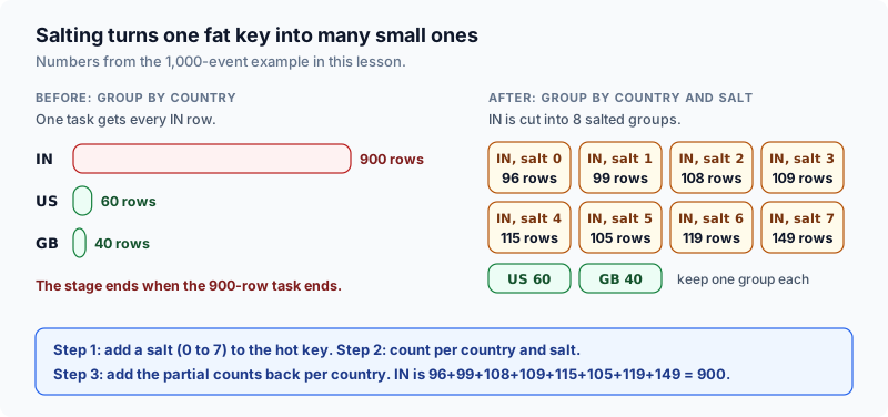
Salting turns one fat key into many small ones.
Did the salt actually balance the partitions?
Shuffle on country plus salt, then count rows per partition again.
(salted.repartition(4, "country", "salt")
    .groupBy(F.spark_partition_id().alias("partition"))
    .count()
    .orderBy("partition")
    .show())
Predict: will the biggest partition drop to 225 rows?
+---------+-----+
|partition|count|
+---------+-----+
|        0|  528|
|        1|  258|
|        2|  115|
|        3|   99|
+---------+-----+
The biggest partition fell from 900 rows to 528. It is better, not perfect: with only 4 partitions, several salts still share one.
Salting helps in proportion to how many partitions can take the pieces.
How do you get the real answer back?
Production salting has 3 steps: add the salt, aggregate on key plus salt, then combine the partials and drop the salt.
partial = salted.groupBy("country", "salt").agg(F.count("*").alias("events"))

final = (
    partial.groupBy("country")
    .agg(F.sum("events").alias("events"))
    .orderBy(F.col("events").desc())
)
final.show()+-------+------+ |country|events| +-------+------+ | IN| 900| | US| 60| | GB| 40| +-------+------+
The totals match the first histogram, so salting changed the work split and not the result.
Aggregate on key plus salt, then drop the salt.
What changes for a join?
Salt the big side the same way. Repeat each row of the small side once per salt value.
This is a sketch and was not run here.
200 shuffle partitions can still leave one task with 90% of the rows if that task owns one fat key. Inspect the largest group, not only spark.sql.shuffle.partitions.
df.groupby('country').size() is the same histogram. pandas will not straggle across machines, but a huge group still blows RAM on one laptop. Spark adds a network shuffle on top of that imbalance.
What is the picture to remember?
Nine loading docks and one pallet that holds 90% of the boxes. Eight crews finish early.
Salt splits that pallet into IN-0 through IN-7, so eight crews lift together.
How does the whole incident replay?
The stage stalls at 99% while one task keeps running.
- stage 99%
- one straggler
Group by the suspect key, count, and sort. IN has 900 of 1,000 rows.
- groupBy country
- IN = 900
Confirm the imbalance: 1 partition holds 900 rows.
- partition 1
- 900 rows
Salt the hot key into 8 groups, aggregate, then drop the salt.
- IN-0 to IN-7
- sum
- IN = 900
Four things to remember:
- Skew is a key with far more rows than its siblings, and the slowest task sets the job time.
- Find it with a histogram: groupBy the key, count, order descending.
- More partitions do not split one fat key. AQE can help, but read the histogram anyway.
- Salt the hot key, aggregate on key plus salt, then combine and drop the salt.
Common beginner questions
Is skew the same as too few partitions?
No. Too few partitions under-uses the cluster even when keys are even. Skew is uneven keys. You can have 400 partitions and still one straggler.
Should I always salt?
No. Salt when a measured key is the bottleneck. Salting complicates the join key. AQE or isolating the hot key into a separate path is often enough.
Where else does this show up?
Cartesian explosions and unfiltered fat scans in Studio are cousins of the same incident: one key or one join ate the job.
What comes next
Once you can see a whale key, you need to see the shuffle itself.
The next lesson reads a Catalyst physical plan with explain().
Practice
Run Sample to see the histogram.
Then complete the exercise: groupBy country on ecommerce_events and count(*) as events.
Assign the full country list to result, not a tiny limit of raw events.
You are practicing the diagnostic, not salting yet. Look at which country is largest.
Going deeper: when salting helps, when it does not, and how to keep answers correct
The lesson above showed a job stalling on one task and a salt that spreads the hot key. 3 questions remain, and they decide whether you use salting well: is this really skew, how big should the salt be, and does the final answer stay correct?
Step 1: confirm it is skew before you fix it
Skew means unequal tasks, not slow tasks.
| What the Spark UI shows | Likely cause | First thing to try |
|---|---|---|
| One task in a stage runs far longer than the median, the rest finish early | Skew: one key or partition holds most rows | Look at row counts per key; then salting, a broadcast join, or adaptive query execution |
| Every task is slow and similar | Not enough parallelism, or simply a lot of data | More partitions or more executors; salting will not help |
| Thousands of tasks that each finish in milliseconds | Too many tiny partitions | Fewer shuffle partitions or coalescing |
| Tasks show a large Spill value | Partitions too big for execution memory | More partitions or more memory per executor |
| One key is NULL on a huge share of rows | NULL join or group keys all land in 1 partition | Filter or handle NULLs separately |
Step 2: see the imbalance in numbers
A hash partitioner sends every row with the same key to the same partition. If one merchant owns 40% of the orders, that partition receives at least 40% of the rows however many reducers you add.
The program below builds 1,000,000 orders where merchant M1 owns about 40%, hashes them into 8 reducer partitions, then repeats with M1 split into 8 salted keys. Predict whether the salted max-to-median ratio drops below 2.
import random, statistics, zlib

random.seed(7)
# 1,000,000 orders. Merchant M1 owns 40% of them. Other merchants share the rest.
rows = [("M1" if random.random() < 0.4 else f"M{random.randint(2, 200)}", 1)
        for _ in range(1_000_000)]
R = 8                                    # number of reducer partitions

def partition(key):
    return zlib.crc32(key.encode()) % R

def load(make_key):
    counts = [0] * R
    for merchant, _ in rows:
        counts[partition(make_key(merchant))] += 1
    return counts

plain = load(lambda m: m)
print("plain :", plain, "max/median", round(max(plain) / statistics.median(plain), 2))

SALT = 8
salted = load(lambda m: f"{m}#{random.randrange(SALT)}" if m == "M1" else m)
print("salted:", salted, "max/median", round(max(salted) / statistics.median(salted), 2))plain : [75411, 78671, 72629, 71953, 71949, 475436, 75205, 78746] max/median 6.31 salted: [125088, 128471, 122814, 121680, 122266, 125431, 125307, 128943] max/median 1.03
Without salt, 1 partition holds about 475,000 rows while the median holds about 76,000, so the job waits for a task 6 times larger than typical. With salt, every partition holds about 125,000. The total work did not change; only the slowest task did.
Step 3: choose a first salt factor with arithmetic
Aim for each salted piece to be about the size of a normal partition. Normal here is 1,000,000 / 8 = 125,000 rows. The hot key has about 400,000 rows. 400,000 / 125,000 is 3.2, so you need at least 4 pieces.
Start with a small power of two such as 4 or 8, measure the max-to-median task time again, and stop when it is close to even. Larger salts cost more: each extra piece is another group that needs a second combine step, and in a join another copy of the other side.
Salting every key multiplies work for keys that were fine. Add the random suffix only when the key is in a short list of hot keys (found with a count by key), and leave the rest unchanged.
Step 4: keep the answer correct
Salting turns one group into several partial groups, which you then combine. That is only correct when the aggregate can be rebuilt from partial pieces. Predict each line before you open the output.
# Which aggregates survive being split across partial results?
amounts = [10, 10, 10, 10, 10, 10, 10, 10, 10, 100]
part_a, part_b = amounts[:9], amounts[9:]          # two salted buckets for one key

print("true average      :", sum(amounts) / len(amounts))
print("average of averages:", (sum(part_a) / len(part_a) + sum(part_b) / len(part_b)) / 2)
print("sum / count       :", (sum(part_a) + sum(part_b)) / (len(part_a) + len(part_b)))

visits = ["u1", "u2", "u3", "u1", "u2", "u3", "u1"]    # user ids seen for one hot key
bucket0, bucket1 = set(visits[0::2]), set(visits[1::2])
print("true distinct users        :", len(set(visits)))
print("sum of per-bucket distincts:", len(bucket0) + len(bucket1))true average : 19.0 average of averages: 55.0 sum / count : 19.0 true distinct users : 3 sum of per-bucket distincts: 6
| Aggregate | Safe to split and recombine? | How to recombine |
|---|---|---|
| SUM, COUNT, MIN, MAX | Yes | Apply the same function to the partial results (sum the sums, add the counts) |
| AVG | Only through its parts | Keep SUM and COUNT per piece, add them, then divide once. Averaging the averages gave 55.0 instead of 19.0 |
| COUNT DISTINCT | No, not by adding | First deduplicate the (key, value) pairs, then count. Adding per-piece distincts gave 6 instead of 3 |
| MEDIAN, exact percentiles | No | Use an approximate method, or a different design that does not need the whole set in one place |
Why plain sums are often already protected
Before a shuffle, Spark combines rows inside each map task (a partial aggregation). For a SUM or COUNT by key, a map task sends 1 row per key instead of every row. Predict how many records cross the network in our 1,000,000-row example with 20 map tasks.
import random
random.seed(7)
rows = [("M1" if random.random() < 0.4 else f"M{random.randint(2, 200)}", 1) for _ in range(1_000_000)]
maps = 20
per_map = len(rows) // maps
no_combine = len(rows)
combined = sum(len({m for m, _ in rows[i * per_map:(i + 1) * per_map]}) for i in range(maps))
print("records shuffled, no combine :", no_combine)
print("records shuffled, map-side :", combined)records shuffled, no combine : 1000000 records shuffled, map-side : 4000
So a hot key in a simple SUM often adds almost nothing to the shuffle. Skew bites hardest in joins, in operations that must see every row of a key together (collect_list, window functions, exact distinct counts), and when the hot key's rows cannot be combined first.
When salting is unnecessary or makes things worse
| Situation | Why salting is the wrong tool | Better first move |
|---|---|---|
| One side of the join is small | A broadcast join copies the small table to every executor, so the big table is never shuffled by key | Broadcast the small side |
| Spark 3 with adaptive query execution on | It can split oversized partitions in a sort-merge join when skew join handling is enabled | Check the setting and the plan before writing salting code |
| The slow key is NULL | NULL is not a real business entity; its rows rarely need to join or group | Filter or route NULL rows separately |
| The dataset is small | The extra stage costs more than the imbalance | Leave it alone |
| You need exact per-key ordering or an exact median | Splitting the key breaks the guarantee | Redesign, or accept an approximate result |
What changes for a join
To salt a join, add a random suffix 0 to S-1 to each hot-key row on the big side. The other side must then contain every suffix, so each of its hot-key rows is copied S times.
A hot key with 400,000 rows on the big side and 1 row on the small side becomes S pieces of about 400,000 / S rows each, and the small side grows from 1 row to S rows for that key. That cost is why S should stay small.
Try a new scenario
You aggregate 10 million rows into 200 shuffle partitions by customer_id. One customer owns 30% of the rows, and the aggregate is the average basket value. Choose a first salt factor and say how you rebuild the average.
Work it out, then open the answer
A normal partition holds 10,000,000 / 200 = 50,000 rows. The hot customer has 3,000,000 rows, so 3,000,000 / 50,000 = 60 pieces would match the normal size. Start lower, for example 16 or 32, and measure, because each extra piece adds merge work. Rebuild the average from parts: keep SUM(basket) and COUNT(*) for each salted piece, add them across pieces, then divide once. Do not average the piece averages.
A teammate says: 'Spark has adaptive execution, so we never need salting.' Fair?
Partly. Adaptive execution helps with skew inside certain joins. It does not rewrite your aggregation logic, handle every operation that needs all rows of a key together, or fix a bad key choice. Check the physical plan and the Spark UI, then decide.
Close the lesson and explain it
Without scrolling up, explain why averaging the averages is wrong, and name one situation where you would broadcast instead of salting.
Practicals · load into the editor
After you read the theory, run these in the pane on the right. They execute in this tab, no cluster.
Finished this lesson?
Mark it as read when you could explain it to someone else.
Practice this
Same ideas as interview drills. These challenges open in the studio with a dataset and tests already set up.